07. Post Perturbation Analysis Tutorial
In this notebook, we examine transcriptomic changes following in silico perturbation. The output of the PerturbGen in-silico module (Notebook 6) is an .h5ad file containing the original input observations, along with a per-cell mean_cos_similarity metric. This metric represents the average cosine similarity of gene embeddings between post-perturbation and pre-perturbation states, where lower values indicate stronger perturbation effects.
The AnnData object includes two additional layers:
pred_counts: reconstructed gene expression counts prior to perturbationtrue_counts: original observed gene expression counts
The perturbed gene expression counts are stored in the main matrix X. These counts are in raw form and should be normalized and log-transformed before downstream analysis.
Load the libraries
import scanpy as sc
import pandas as pd
import numpy as np
import seaborn as sns
import matplotlib.pyplot as plt
import os
import re
import gseapy as gp
Load the .h5ad object containing the results of the post–in silico perturbation.
adata = sc.read('/path/to/in-silico/anndata.h5ad') # e.g. 20250812-13:47_minference_adata_gENSG00000125538_ssrc_tmask.h5ad
As noted earlier, perturbed gene expression counts are stored in .X, while unperturbed (predicted) counts are stored in layers['pred_counts']. To organize these data, we construct a new AnnData object with the following annotations:
status: indicates whether a cell is perturbed or unperturbedstatus_time: records the perturbation status at each timepoint
pred = adata.copy()
pred.X = pred.layers['pred_counts'].copy()
pred.obs['status'] = 'unperturbed'
adata.obs['status'] = 'perturbed'
adata.obs['status_time'] = 'perturbed_' + adata.obs['time_after_LPS'].astype(str)
pred.obs['status_time'] = 'unperturbed_' + pred.obs['time_after_LPS'].astype(str)
adata = adata.concatenate(pred) # combine perturbed and unperturbed data
/tmp/ipykernel_758363/3760186430.py:1: FutureWarning: Use anndata.concat instead of AnnData.concatenate, AnnData.concatenate is deprecated and will be removed in the future. See the tutorial for concat at: https://anndata.readthedocs.io/en/latest/concatenation.html
  adata = adata.concatenate(pred)
The predicted counts for both the unperturbed and perturbed conditions are stored in their raw form. Therefore, it is necessary to normalize and log-transform these counts prior to downstream analyses.
sc.pp.normalize_total(adata) # normalize total counts per cell
sc.pp.log1p(adata) # log-transform the data
Optionally, We renamed the cell types for consitency.
mapping = {
    'B cell': 'B cells',
    'CD14 monocytes': 'CD14+ monocytes',
    'CD16 monocytes': 'CD16+ monocytes',
    'CD4+ T cells': 'CD4+ T cells',
    'CD8+ T cells': 'CD8+ T cells',
    'Dendritic cells': 'Dendritic cells',
    'NK': 'NK cells',
    'NKT': 'NKT cells',
    'Plasmocytoid dendritic cell': 'Plasmacytoid dendritic cells',
    'hematopoietic stem cell': 'Hematopoietic stem cells',
    'platelet': 'Platelets'
}

adata.obs['cell_type_harmonized'] = adata.obs['cell_type_harmonized'].cat.rename_categories(
    {cat: mapping.get(cat, cat) for cat in adata.obs['cell_type_harmonized'].cat.categories}
)
Here, we evaluate the number of significant differentially expressed genes (DEGs) for each cell type by comparing perturbed counts with unperturbed counts. We refer to this measure as the perturbation effect.
cell_types = adata.obs['cell_type_harmonized'].unique()
timepoints = ['6h_LPS', '10h_LPS']
results = []

for tp in timepoints:
    unperturbed = f'unperturbed_{tp}'
    perturbed   = f'perturbed_{tp}'

    for ct in cell_types:
        mask_pert = (adata.obs['status_time'] == perturbed) & (adata.obs['cell_type_harmonized'] == ct)
        mask_unpt = (adata.obs['status_time'] == unperturbed) & (adata.obs['cell_type_harmonized'] == ct)

        if mask_pert.sum() == 0 or mask_unpt.sum() == 0:
            continue

        sub_adata = adata[mask_pert | mask_unpt].copy()
        sub_adata.obs['group'] = 'unperturbed'
        sub_adata.obs.loc[sub_adata.obs['status_time'] == perturbed, 'group'] = 'perturbed'
        sub_adata.obs['group'] = sub_adata.obs['group'].astype('category')

        sc.tl.rank_genes_groups(sub_adata, groupby='group', reference='unperturbed',method='wilcoxon')
        degs = sc.get.rank_genes_groups_df(sub_adata, group='perturbed')
        deg_count = (degs['pvals_adj'] < 0.05).sum()
        results.append({'cell_type': ct, 'timepoint': tp, 'deg_count': deg_count})

df = pd.DataFrame(results)
df_sorted = df.sort_values(by='deg_count', ascending=False)
df_sorted['timepoint'] = df_sorted['timepoint'].replace({
    '6h_LPS': '6h',
    '10h_LPS': '10h'
})
sns.set_context("talk", font_scale=1.2)
plt.figure(figsize=(8, 6))
sns.barplot(data=df_sorted, y='cell_type', x='deg_count', hue='timepoint')
plt.ylabel('Cell type', fontsize=16)
plt.xlabel('DEGs count', fontsize=16)
plt.title('Perturbation effect', fontsize=16)
plt.xticks(fontsize=12)
plt.yticks(fontsize=12)
plt.legend(title='Timepoint', fontsize=14, title_fontsize=16)
plt.tight_layout()
plt.show()
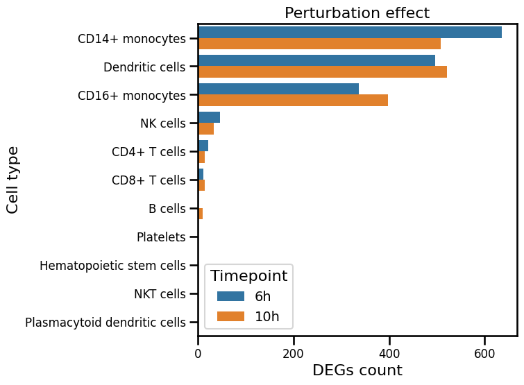
Next, we subset the data to the myeloid lineage, which exhibits the strongest perturbation effect. Depending on the analysis goals, the data can alternatively be subset to any other affected cell types or lineages of interest.
adata = adata[adata.obs['cell_type_harmonized'].isin(['CD14 monocytes','Dendritic cells',
                                                     'CD16 monocytes'])].copy()
Because the var_names in the AnnData object are stored as Ensembl IDs, we reload the original dataset to obtain the mapping needed to convert them into gene symbols.
adata_full = sc.read('/path/to/full/anndata.h5ad')
Since the original reference data is raw, we need to normalize and log-transform it before we can compare it with other results.
sc.pp.normalize_total(adata_full) # normalize the data
sc.pp.log1p(adata_full) # log-transform the data
We convert the var_names in the original object from gene symbols to their corresponding Ensembl IDs.
adata_full.var_names = adata_full.var['ensembl_id-0'] # set gene names to Ensembl IDs
Since the var_names in the perturbation object are stored as Ensembl IDs, we map them to their corresponding gene symbols using the original object.
mapping = adata_full.var['gene_ids-0'].to_dict()
adata.var_names = adata.var_names.map(mapping) # map gene names to full data
adata = adata[:, adata.var_names.notnull()].copy() # keep only genes present in full data
We next calculate the DEGs within the myeloid lineage, as this lineage showed the strongest response to perturbation. Specifically, we compute DEGs at each timepoint by comparing perturbed counts against the unperturbed counts (used as reference). From this, we identify upregulated and downregulated DEGs separately for each timepoint, which are then used for enrichment analysis.
deg_results = {}

for tp in ["6h", "10h"]:
    pert = f"perturbed_{tp}_LPS"
    unpert = f"unperturbed_{tp}_LPS"

    ad = adata[adata.obs["status_time"].isin([pert, unpert])].copy()
    ad.obs["cond"] = ad.obs["status_time"].map({pert: "pert", unpert: "unpert"}).astype("category")

    sc.tl.rank_genes_groups(ad, groupby="cond", groups=["pert"], reference="unpert",
                            method="wilcoxon", corr_method="benjamini-hochberg")

    de = sc.get.rank_genes_groups_df(ad, group="pert")

    sig = de[(de["pvals_adj"] < 0.05)]
    up = sig[sig["logfoldchanges"] > 0]
    down = sig[sig["logfoldchanges"] < 0]
    deg_results[tp] = {"up": up["names"].tolist(), "down": down["names"].tolist()}
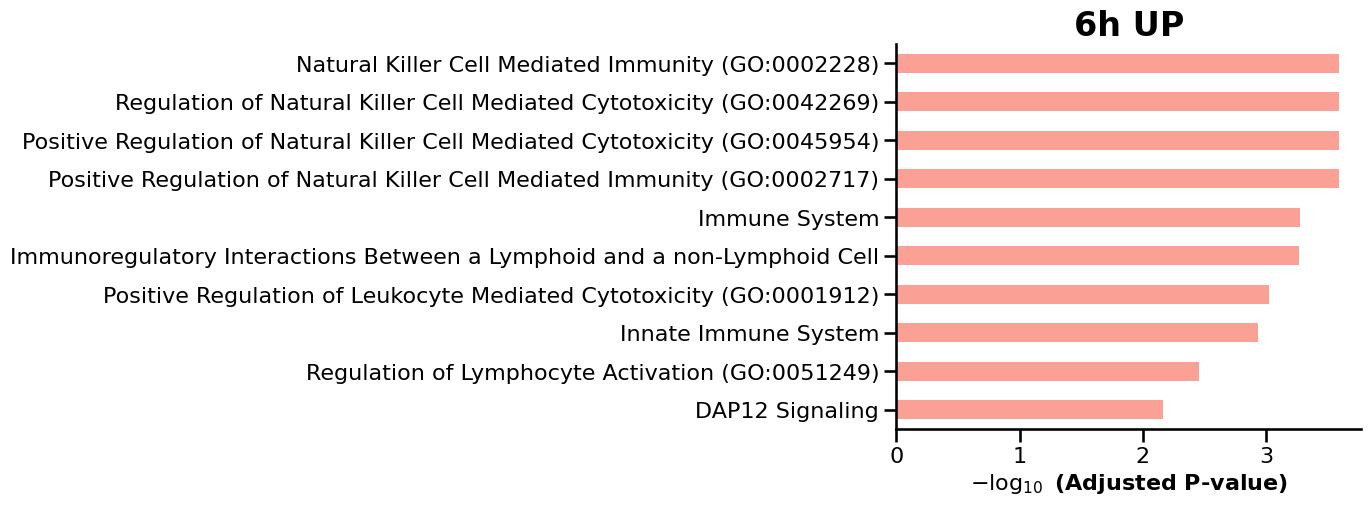
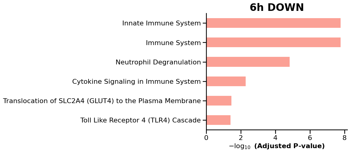
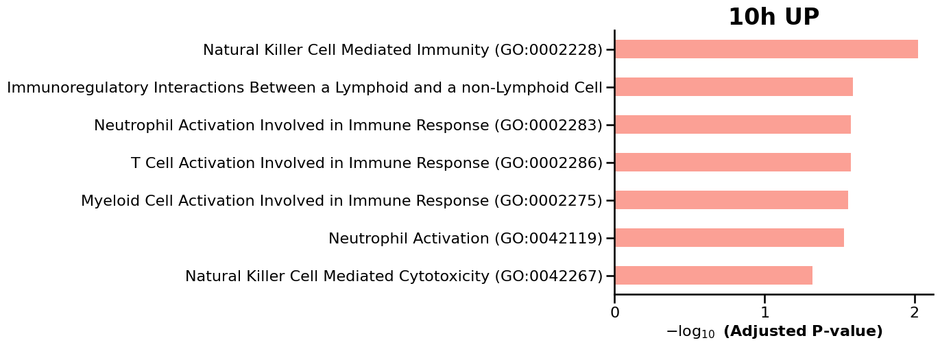
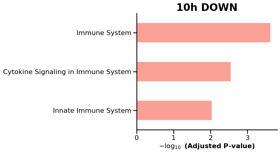
We then use GSEApy to perform enrichment analysis on the differentially expressed genes (DEGs) identified at each timepoint, enabling the identification of enriched biological pathways and gene sets over time. ref: GSEApy is a Python implementation of Gene Set Enrichment Analysis (Fang et al., 2023).
for tp, res in deg_results.items():
    for label, genes in res.items():
        if len(genes) == 0:
            continue

        enr = gp.enrichr( # perform enrichment analysis
            gene_list=genes,
            gene_sets=["Reactome_Pathways_2024","GO_Biological_Process_2025"],
            organism="Human",
            outdir=None,
            background = list(adata.var_names) ,
        )

        df = enr.results.sort_values("Adjusted P-value").head(15)

        ax = gp.barplot(df, column="Adjusted P-value", title=f"{tp} {label.upper()}", figsize=(6, 5))
        plt.show()